Components Of Time Series
Aug 13, 2024
Components of Time Series
The components of time series data are the underlying patterns or structures that make up the data. There are several common components in time series data:
Trend
A trend in time series data refers to a long-term upward or downward movement in the data, indicating a general increase or decrease over time. The trend represents the underlying structure of the data, capturing the direction and magnitude of change over a longer period. There are several types of trends in time series data:
Upward Trend: A trend that shows a general increase over time, where the values of the data tend to rise over time.
Downward Trend: A trend that shows a general decrease over time, where the values of the data tend to fall over time.
Linear Trend: A trend that can be approximated by a straight line.
Non-linear Trend: A trend that cannot be approximated by a straight line and follows a curved pattern.
Here's an example of how to visualize a time series with a trend in Python using the Matplotlib library:
This code generates a time series with a linear upward trend and some random noise.
Seasonality
Seasonality refers to a repeating pattern in the data that occurs at regular intervals, such as daily, weekly, monthly, or yearly. Seasonal patterns are often caused by external factors, such as weather, holidays, or business cycles. For example, ice cream sales typically have a seasonal pattern, with higher sales during the summer months and lower sales during the winter months.
Here's an example of how to generate a time series with seasonality in Python using the NumPy library:
This code generates a time series with a sinusoidal seasonal pattern and some random noise.
Cyclicality
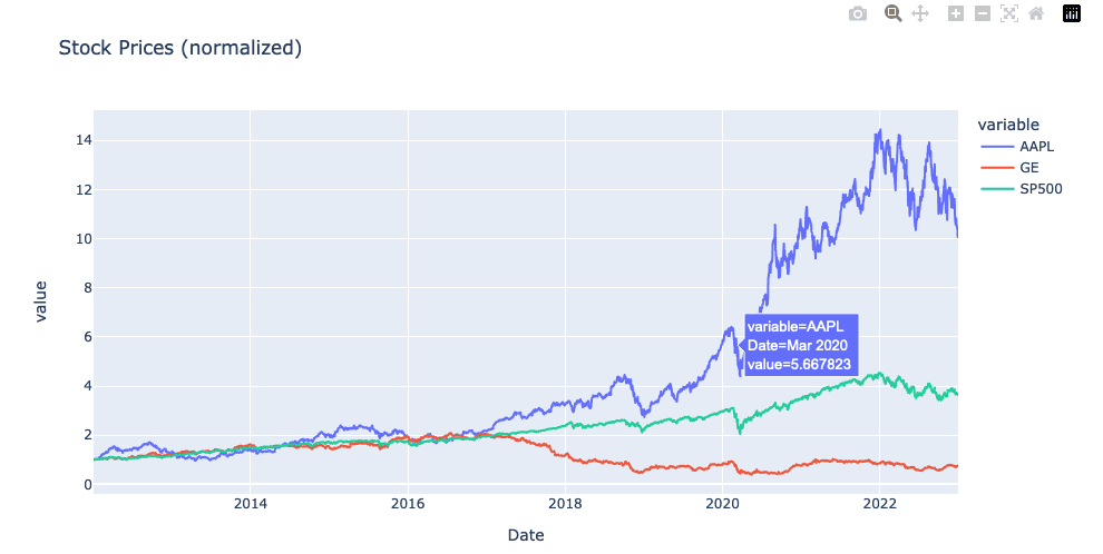
Cyclicality refers to irregular patterns in the data that are not periodic but repeating over a more extended period. Cyclical patterns are often caused by economic factors, such as business cycles or market trends. For example, the stock market often exhibits cyclical patterns, with periods of growth followed by periods of decline.
Irregularity
Irregularity refers to random fluctuations in the data that cannot be easily explained by trend, seasonality, or cyclicality. These fluctuations are often caused by unpredictable events or measurement errors. Irregularity can make it difficult to identify patterns in the data and can affect the accuracy of forecasts. Here's an example of how to generate a time series with irregularity in Python using the NumPy library:
This code generates a time series with random fluctuations using the np.random.rand() function.
Autocorrelation
Autocorrelation is a measure of how correlated a time series is with itself at different lags. Autocorrelation can help identify the presence of patterns and relationships in the data. A time series with significant autocorrelation at a particular lag suggests that the previous observations at that lag are related to the current observation.
Here's an example of how to generate a time series with autocorrelation in Python using the NumPy library:
This code generates a time series with autocorrelation by applying a moving average filter to the data.
Outliers
Outliers in time series data are data points that are significantly different from the rest of the data points in the series. These can be due to various reasons such as measurement errors, extreme events, or changes in underlying data-generating processes. Outliers can have a significant impact on the results of time series analysis and modeling, as they can skew the statistical properties of the data.
Noise
Noise in time series data refers to random fluctuations or variations that are not due to an underlying pattern or trend. It is typically considered as any unpredictable and random variation in the data. These fluctuations can arise from various sources such as measurement errors, random fluctuations in the underlying process, or errors in data recording or processing. The presence of noise can make it difficult to identify the underlying trend or pattern in the data, and therefore it is important to remove or reduce the noise before any further analysis.
Time Series Analysis
Time series analysis is a statistical technique that uses historical data points to predict future trends and patterns. This technique is based on the assumption that future trends and patterns are influenced by past events and behavior. The primary goal of time series analysis is to identify patterns and trends in data over time.
Time series analysis can be used to forecast sales, stock prices, and other variables. It can also be used to identify the underlying causes of changes in a variable over time. For example, time series analysis can be used to identify the factors that influence the price of a particular commodity, such as supply and demand, weather patterns, or political events. Here's an example of how to import and visualize time series data in R using the ggplot2 library:
Time Series Forecasting
Time series forecasting means assessing the time-stamped data using statistical calculations and modeling to make predictions and induce strong strategic decision-making. The process is widely adopted in many sectors, for example, sales forecasting and weather forecasting. Forecasting highly depends on the nature of the data, and the process is usually performed on historical data. The more simplified it is, the more accurate the forecasting becomes.
The model does have its limitations as it does not guarantee accuracy and may vary from the actual outcome. However, the analysts have some operating authority over models to regulate such constraints. Examples of time series methods used for forecasting are Autoregression (AR), Moving Average (MA), Autoregressive Moving Average (ARMA), and Autoregressive Integrated Moving Average (ARIMA).
Conclusion
In conclusion, time series data can be decomposed into several components, including trend, seasonality, cyclicity, irregularities, autocorrelation, outliers, and noise. Understanding these components is crucial for analyzing and modeling time series data effectively. By identifying and isolating these components, we can gain a better understanding of the underlying patterns and relationships in time series data, which can inform decision-making and improve forecasting accuracy.