Introduction to Multilayer Networks in Machine Learning
Aug 14, 2024
In this comprehensive blog post, we will delve into the intricacies of multilayer networks, exploring their architecture, functionalities, and applications. We will begin by establishing a solid foundation in neural network fundamentals, gradually progressing to dissect the anatomy of an MLP and comprehensively understanding its mechanisms. From forward propagation to backpropagation, we'll navigate through the essential algorithms driving the training and optimization of MLPs.
Furthermore, we'll explore the diverse landscape of activation functions, crucial elements that dictate the behaviour and expressiveness of MLPs. Through practical examples and theoretical discussions, we'll shed light on the strengths and limitations of various activation functions, empowering you to make informed choices in model design.
Understanding Single-layer Artificial Neural Networks (ANN)
Before we dive into the world of multilayer networks, it's essential to understand the basic building blocks of neural networks: single-layer Artificial Neural Networks (ANN), also known as single-layer perceptrons. These networks consist of interconnected input and output nodes, each with its own weight.
In a single-layer ANN, the input nodes receive data or information, which is then processed through the network's weights. The output nodes generate the final result or prediction based on the weighted sum of the inputs. The weights in a single-layer ANN are crucial as they determine the strength and importance of each input in producing the output. During training, the weights are adjusted to optimize the network's performance and accuracy, typically using algorithms like gradient descent.However, single-layer ANNs have limitations. They can only solve linearly separable problems, where the data can be classified into distinct categories using a straight line or a hyperplane. These networks struggle with complex patterns and non-linear relationships between inputs and outputs.
The Rise of Multilayer Perceptrons (MLPs)
To overcome the limitations of single-layer ANNs, researchers introduced the concept of multilayer neural networks. The addition of hidden layers between the input and output nodes enabled these networks to learn and recognize subtle patterns in data. This architectural development gave rise to the Multilayer Perceptron (MLP), a form of neural network that has since gained widespread recognition and use in a variety of applications.
The interest in MLPs neural networks skyrocketed in the 1990s. Pattern recognition, image processing, natural language processing, and financial forecasting were all investigated by researchers and practitioners. However, the restricted processing capacity and availability of big datasets created hurdles to the broad implementation of MLPs throughout this period.
MLP deep learning architectures underwent a revival in the twenty-first century, thanks to advances in processing technology and the introduction of big data. Researchers were able to train deep neural networks with numerous layers because of the availability of enormous quantities of data and the development of powerful GPUs, resulting in amazing discoveries in fields such as computer vision, voice recognition, and autonomous systems.MLPs are still used in deep learning and machine learning applications today. Their capacity to deal with complicated patterns, nonlinear interactions, and large-scale datasets has made them indispensable in tackling real-world issues in a variety of disciplines.
Anatomy of a Multilayer Perceptron
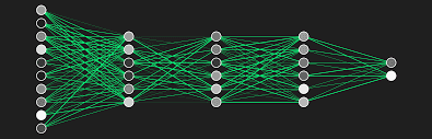
The Multilayer Perceptron (MLP) is at the heart of multi-layer neural networks. An MLP is a multi-layer feedforward neural network having input, hidden, and output layers. The hidden layers are in charge of collecting and learning complicated patterns in data, allowing MLPs to solve nonlinear problems.
The MLP architecture is characterized by interconnected nodes, or neurons, in each layer. Each neuron receives inputs, which are multiplied by corresponding weights and summed. An activation function is then applied to the sum to introduce non-linearity and produce the output of the neuron. This process is repeated for all neurons in each layer, propagating the information forward through the network. Here's a simple example of an MLP implementation in Python using the NumPy library:
In this example, we define an MLP with an input layer of size 10, a hidden layer of size 20, and an output layer of size 5. We initialize the weights and biases randomly and define a sigmoid activation function. The forward function performs the forward propagation through the network, applying the activation function to the weighted sum of inputs at each layer.
Forward Propagation in MLPs
Forward propagation is a fundamental process in neural networks, including Multilayer Perceptrons (MLPs), where input data is sequentially passed through the network layers to produce an output prediction.The forward propagation process in an MLP can be summarized as follows:
Input Data Transmission: Forward propagation begins by feeding the input data into the first layer of the MLP.
Weighted Sum Computation: For each neuron in a layer, the inputs are multiplied by their corresponding weights and summed, including a bias term.
Activation Function Application: An activation function is applied to the weighted sum to introduce non-linearity and produce the output of the neuron.
Layer-wise Propagation: The outputs of the current layer become the inputs for the next layer, and the process is repeated until the final output layer is reached.
Output Generation: The output of the MLP is the result of the forward propagation process, representing the network's prediction or decision based on the input data.
The choice of activation function plays a crucial role in the expressiveness and performance of an MLP. Some commonly used activation functions include:
Sigmoid: σ(x)=11+e−xσ(x)=1+e−x1
Tanh: tanh(x)=ex−e−xex+e−xtanh(x)=ex+e−xex−e−x
ReLU (Rectified Linear Unit): ReLU(x)=max(0,x)
Leaky ReLU: LeakyReLU(x)={xif x≥0αxif x<0LeakyReLU(x)={xαxif x≥0if x<0
Each activation function has its own characteristics and is suitable for different types of problems and network architectures.
Backpropagation and Training of MLPs
The training of an MLP is typically done using the backpropagation algorithm, which allows the network to learn from its mistakes and improve its performance over time. Backpropagation involves two main steps:
Forward Propagation: Input data is passed through the network to generate output predictions, as described in the previous section.
Backward Propagation: The computed gradients are then propagated backwards through the network, starting from the output layer and moving towards the input layer. At each layer, the gradients are used to update the parameters (weights and biases) of the network using an optimization algorithm like gradient descent or its variants (e.g., stochastic gradient descent, Adam optimizer). The magnitude of the parameter updates is determined by the learning rate, which controls the step size in the parameter space.
The backpropagation algorithm can be summarized as follows:
In this example, we compute the error at the output layer using the difference between the predicted output and the true output. We then backpropagate the error to the hidden layer using the transpose of the weights. Finally, we update the weights and biases using the computed gradients and the learning rate.
Applications of MLPs in Machine Learning
MLPs have found applications in a wide range of domains, showcasing their versatility and effectiveness in solving complex problems. Here are a few examples:
Image Recognition: MLPs have been successfully applied to image classification tasks, where they learn to recognize patterns in pixel data and assign labels to images.
Natural Language Processing: MLPs are used in various NLP tasks, such as text classification, sentiment analysis, and language modeling, by learning representations of words and sentences.
Financial Forecasting: MLPs can be trained on historical financial data to predict stock prices, forecast market trends, and make investment decisions.
Bioinformatics: MLPs have been used in bioinformatics for tasks like protein structure prediction, gene expression analysis, and drug discovery.
Robotics and Control Systems: MLPs are employed in robotics for control and decision-making, enabling robots to navigate complex environments and perform tasks autonomously.
Limitations and Challenges of MLPs
While MLPs have proven to be powerful tools in machine learning, they also face certain limitations and challenges:
Overfitting: MLPs with a large number of parameters can easily overfit the training data, leading to poor generalization performance on unseen data. Regularization techniques, such as L1/L2 regularization, dropout, and early stopping, are used to mitigate overfitting.
Vanishing/Exploding Gradients: In deep MLPs with many layers, the gradients computed during backpropagation can either vanish (become extremely small) or explode (become extremely large), making it difficult to train the network effectively. Techniques like batch normalization and residual connections have been developed to address this issue.
Interpretability: MLPs, especially deep architectures, are often considered "black boxes" due to their complexity and the difficulty in interpreting the learned representations. Efforts are being made to develop more interpretable and explainable neural network models.
Computational Complexity: Training MLPs can be computationally expensive, especially for large datasets and deep architectures. The use of GPUs and distributed computing has helped speed up the training process, but it remains a challenge for certain applications.
Conclusion
In this blog post, we've explored the fascinating world of multilayer networks in machine learning, delving into the intricacies of Multilayer Perceptrons (MLPs). From understanding the fundamentals of neural networks to dissecting the anatomy of MLPs and exploring training strategies and regularization techniques, we've covered many topics essential for mastering this powerful machine-learning tool.
MLPs have demonstrated remarkable versatility and effectiveness across various domains, from image classification and natural language processing to time series forecasting. Their ability to capture complex patterns and relationships in data makes them indispensable in the modern machine learning landscape.