Introduction to Time Series in Machine Learning
Aug 13, 2024
Time series data is a sequence of observations collected over time at regular intervals, such as daily, weekly, or monthly. In contrast to cross-sectional data, where observations are independent of each other, time series data exhibits temporal dependencies and patterns that are crucial for analysis and forecasting. Machine learning has revolutionized the field of time series analysis, enabling us to uncover complex patterns, trends, and relationships within the data.
In this comprehensive blog post, we will dive into the world of time series in machine learning, exploring its concepts, techniques, and applications. We will discuss the challenges of working with time series data, the key components that characterize it, and the various machine learning algorithms used for time series forecasting. Additionally, we will provide practical examples and code snippets to illustrate the implementation of these techniques.
Understanding Time Series Data
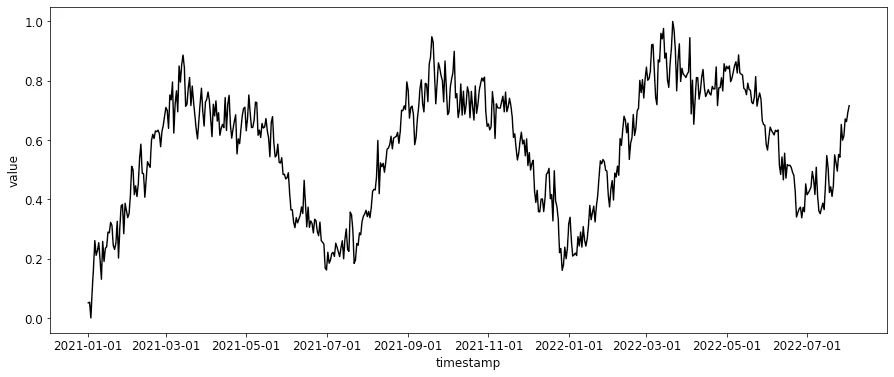
Time series data consists of observations recorded at regular intervals over time. It can be represented as a sequence of values, where each value corresponds to a specific time point. The order and temporal dependencies between observations are essential in time series data, as they can reveal valuable insights and patterns. Time series data can be characterized by several key components:
Trend: A long-term increase or decrease in the data over time, often represented by a
linearornon-linear function.Seasonality: Recurring patterns that occur within specific time frames, such as daily, weekly, monthly, or yearly cycles.
Cyclicity: Repetitive changes in the time series that do not necessarily occur at fixed intervals.
Irregularity/Noise: Random fluctuations or unpredictable variations in the data that cannot be explained by the other components.
Understanding these components is crucial for effectively modeling and forecasting time series data using machine learning techniques.
Challenges in Working with Time Series Data
While time series data offers valuable insights, it also presents several challenges that need to be addressed when applying machine learning techniques:
Handling missing values: Time series data may contain missing observations due to various reasons, such as sensor failures or data collection errors. Imputation techniques are used to estimate the missing values based on the surrounding data points.
Dealing with non-stationarity: Time series data may exhibit non-stationarity, meaning that the statistical properties of the data change over time. This can be caused by trends, seasonality, or other external factors. Non-stationarity needs to be addressed before applying certain machine learning algorithms.
Capturing complex patterns: Real-world time series data can exhibit complex patterns, such as multiple seasonalities, interactions between components, or non-linear relationships. Machine learning models need to be flexible enough to capture these intricate patterns.
Evaluating model performance: Assessing the performance of time series models is different from traditional machine learning tasks due to the temporal dependencies in the data. Metrics like mean squared error (MSE) or mean absolute percentage error (MAPE) are commonly used for evaluating time series forecasting models.
Incorporating external factors: Time series data can be influenced by various external factors, such as weather conditions, economic indicators, or social events. Incorporating these factors into the machine learning models can improve the accuracy of forecasts.
Machine Learning Techniques for Time Series Forecasting
Machine learning offers a wide range of techniques for time series forecasting, each with its own strengths and weaknesses. Here are some of the most popular methods:
1. Autoregressive Integrated Moving Average (ARIMA)
ARIMA is a classical statistical model that combines autoregressive (AR) and moving average (MA) components. It is suitable for modeling and forecasting time series data with trends and seasonality. The ARIMA model can be expressed as:
where p, d, and q represent the order of the AR, differencing, and MA components, respectively.
2. Recurrent Neural Networks (RNNs)
RNNs are a type of neural network designed to handle sequential data, such as time series. They can learn patterns and dependencies within the data by maintaining a hidden state that is updated at each time step. RNNs are particularly useful for modeling long-term dependencies in time series data.
3. Long Short-Term Memory (LSTM) Networks
LSTMs are a specific type of RNN that are designed to handle long-term dependencies more effectively. They use memory cells and gates to control the flow of information, allowing them to capture complex patterns in time series data.
4. Convolutional Neural Networks (CNNs)
CNNs are primarily used for processing spatial data, such as images. However, they can also be applied to time series data by treating the temporal dimension as the "channels" in an image. CNNs are effective at capturing local patterns and features in time series data.
5. Ensemble Methods
Ensemble methods involve combining multiple models to improve the accuracy of forecasts. Some popular ensemble techniques for time series forecasting include:
Bagging: Training multiple models on different subsets of the data and averaging their predictions.
Boosting: Training models sequentially, where each subsequent model focuses on correcting the errors of the previous model.
Stacking: Training a meta-model to learn how to combine the predictions of multiple base models.
Conclusion
Time series in machine learning is a powerful tool for analyzing and forecasting sequential data. By understanding the key components of time series data and applying appropriate machine learning techniques, we can uncover valuable insights and make informed decisions. As technology continues to advance, the field of time series forecasting will likely see further advancements, enabling even more accurate and reliable predictions.